Mastering Financial Analysis of Value Investing with Python for Better Investment Decisions in Taiwan Exchange Market — (2)
Long-term Dupont analysis & Stock Selection Strategy
Investing Stock is a necessary task, after you realise that the money you deposit in bank is getting smaller and smaller due to inflation. Nonetheless, did I invest the right stock? How can I make ourselves feel at ease? I believe financial analyses can definitely help with that. Therefore, here we propose a framework of value investing and also build a practical work flow step-by-step. Stay tuned! Let’s dive in!
These analyses aim for effective long-term investment rather than swing trading.
- Choose worth investing companies at present
- Allocate personal asset into stock market.
This is the 2nd article in the series. To have an introduction and practical exercise of DuPont analysis for single stock please visit here.
Comparison among stocks
Since we have generated a long-term DuPont analysis, it is doable to make endless long-term DuPont analyses. To do so, we first wrap up the process into a function. Like here
from FinMind.data import DataLoader
import pandas as pd


def Dupont_analysis(candidate,quarter='',year=''):
    # connect to api
    api = DataLoader()

    quarters = {'Q1':'03-31','Q2':'06-30','Q3':'09-30','Q4':'12-31'}

    # embedded functions: profit margin, total asset turnover, financial leverage
    def profit_margin(IncomeAfterTaxes, Revenue):
        return IncomeAfterTaxes/Revenue

    def total_asset_turnover(Revenue,TotalAssets):
        return Revenue/TotalAssets

    def financial_leverage(TotalAssets,Equity):
        return TotalAssets/Equity

    # data access via API
    balance_sheet = api.taiwan_stock_balance_sheet(
        stock_id=candidate,
        start_date='2000-01-31',
    )

    financial_statements = api.taiwan_stock_financial_statement(
        stock_id=candidate,
        start_date='2000-01-31',
    )


    df = pd.concat([balance_sheet,financial_statements],axis=0)

    # date intersect: find the dates where all variables are available
    IAF_date = set(df[df['type'].str.contains('IncomeAfterTax')]['date'].values)
    R_date = set(df[df['type'].str.contains('Revenue')]['date'].values)
    TA_date = set(df[df['type'].str.contains('TotalAssets')]['date'].values)
    date_range = sorted(IAF_date & R_date & TA_date)

    # assemble and calculate time-series Dupont analysis
    Dupont = pd.DataFrame({'quarter':[],'profit_margin':[],'total_asset_turnover':[],'financial_leverage':[],'ROE':[]})
    for d in date_range:
        IncomeAfterTaxes = df[(df['type']=='IncomeAfterTaxes') & (df['date'] == d)]['value'].values[0]
        Revenue = df[(df['type']=='Revenue') & (df['date'] == d)]['value'].values[0]
        TotalAssets = df[(df['type']=='TotalAssets') & (df['date'] == d)]['value'].values[0]
        Equity = df[(df['type']=='Equity') & (df['date'] == d)]['value'].values[0]
        pm = profit_margin(IncomeAfterTaxes,Revenue)
        tat = total_asset_turnover(Revenue,TotalAssets)
        fl = financial_leverage(TotalAssets,Equity)
        df_single = pd.DataFrame({'quarter':[d],'profit_margin':[pm],'total_asset_turnover':[tat],'financial_leverage':[fl],'ROE':[pm*tat*fl* 100]})
        Dupont = pd.concat([Dupont,df_single])
    Dupont.insert(loc=0, column='stock id', value=candidate)
    return Dupont
On top of that, we can easily code few lines to get our result. Just like:
stock_id = '2330'
Du_2330 = Dupont_analysis(stock_id)
Du_2330.head(5)
Few lines more to plot a line & bar graph for long-term DuPont Analysis
Dupont_plot = Du_2330.melt(id_vars='quarter')
for i in range(len(Dupont_plot)):
    for key,value in quarters.items():
        if Dupont_plot['quarter'][i][-5:] == value:
            Dupont_plot['quarter'][i] = Dupont_plot['quarter'][i][:4] + '\n' +  key
bar = Dupont_plot[Dupont_plot['variable'] != 'ROE'][Dupont_plot['variable'] != 'stock id']
line = Dupont_plot[Dupont_plot['variable'] == 'ROE']
sns.set_style("whitegrid")

# plot line graph on axis #1
plt.figure(figsize=(40,16))
plt.xticks(fontsize=8,rotation=30)
ax1 = sns.barplot(
    x='quarter',
    y='value',
    hue='variable',
    data=bar,
)
ax1.set_ylabel('')
ax1.set_xlabel('')
ax1.legend(loc="upper left")
ax1.set_ylim(round(min(bar.value)-0.5), round(max(bar.value)+3.5))
# set up the 2nd axis
ax2 = ax1.twinx()
# plot bar graph on axis #2
sns.lineplot(
    x='quarter',
    y='value',
    data=line,
    color='darkred',
    ax = ax2       # Pre-existing axes for the plot
)
ax2.grid(b=False) # turn off grid #2
ax2.set_ylabel('ROE (%)')
ax2.set_ylim(min(line.value)-2, max(line.value)+2)
ax2.legend(['ROE (%)'], loc="upper right")
#plt.savefig(f'img/Dupont_trend_2330.png',dpi=300)
plt.show()
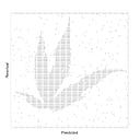
Normal distribution in historical ROE
Looking at the line in the graph, the fluctuation seems to be quite a balance. Therefore, we create a qqplot and conduct a normal test, in order to know if ROE in stocks obeys normal distribution (Fig 2.). The quantile of ROE (blue points) increase along with the mid line (red line), indicating ROE is normal distributed.
norm_roe = (Du_2330.ROE-min(Du_2330.ROE))/(max(Du_2330.ROE)-min(Du_2330.ROE))
k2, p = stats.normaltest(norm_roe)
print(f's^2 + k^2:{k2},\np-value:{p}')
lineStart, lineEnd = 0,1
plt.figure()
plt.scatter(sorted(norm_roe),np.linspace(0,1,len(norm_roe)))
plt.title(label='qq-plot')
plt.plot([lineStart, lineEnd], [lineStart, lineEnd], color = 'r')
#plt.savefig(f'img/qqplot_ROE_2330.png',dpi=300)
Subsequently, we are allowed to calculate mean of ROE and create a 95% confidential interval (CI) unbiasedly. These features (mean & CI) are telling us the expected average ROE and the uncertainty of ROE of a company, which are both crucial for our selection strategy.
pm_mean = np.mean(Du_2330.ROE)
upperCI,lowerCI = pm_mean+2*np.std(Du_2330.ROE), pm_mean-2*np.std(Du_2330.ROE)
Produce a ready-to-campare dataset
So far, we are ready to compare different stocks using DuPont Analysis. Since we have wrapped everything up into a function. Basically, we call a for-loop and concatenate DuPont analyses into a data frame. Thus, we download a ETF0050 list and iterate the DuPont analysis for the stocks on the list. You can find and download the data list here.
today = datetime.today().strftime('%Y-%m-%d')

# import ETF0050 list
eft0050 = pd.read_csv('0050-20220106.csv',sep=';',header=1)
candidate_stocks = eft0050['Stock ID'].apply(lambda x: str(x)).values

# concatenate a list with historical Dupont analyses throughout candidate stocks
df = pd.DataFrame()
for stock in tqdm(candidate_stocks):
    try:
        df_dup = Dupont_analysis(stock)
        df = pd.concat([df,df_dup],axis=0)
    except IndexError or JSONDecodeError:
        time.sleep(1)
        print(f'not sufficient data for {stock}')
Through running long-term Dupont analysis of our target investment (in here the selected stocks in ETF0050), a database containing every record from 2000–01 til now (2023–03) has been maded.
# produce raw dupont analysis dataframe
df_du = df.sort_values('ROE',ascending=False).reset_index(drop=True)
df_du.to_csv(f'dupont_analysis_raw_{today}.csv',index=False)

df_du.head(5)You can make your own to the nearest present date or you can just download the file I made (dupont_analysis_raw_2023–02–27.csv), preferable for your data-analysis skill.
Furthermore, to easily compare, we aggregate/concentrate long-term DuPont analysis data into a single row profile for each stock. We simply calculate the mean and a 95% CI since ROE obeys normal distribution.
(here to download: dupont_analysis_stat_2023–02–27.csv)
# aggregated dupont analysis dataframe
df_aggr = df_du.groupby(by='stock id').mean()
df_std = df_du.groupby(by='stock id').std()['ROE']
df_aggr['UpperCI ROE'] = df_aggr['ROE'] + 2*df_std
df_aggr['LowerCI ROE'] = df_aggr['ROE'] - 2*df_std
df_aggr.sort_values('ROE',ascending=False).to_csv(f'dupont_analysis_stat_{today}.csv')

df_aggr.head(5)
Stock Selection Strategy
Until now, the information is quite clear and rather sufficient for us to make decision. For example, we look up for positive ROE and also low uncertainty (short range of [LowerCI ROE, UpperCI ROE]. For example, interestingly, the highest ROE stocks seem not reliable because the variation. Only 2330 & 2395 have a stability ROE where the confidence intervals are shorter than 6%, and ‘9910’, ’3008', ’2330', ’2395', ’5871' seem to have consistently positive performance throughout years at the top 15.
As a result, we choose 5 stocks ‘9910’, ’3008', ’2330', ’2395', ’5871' to be our final target stocks because we believe great performance and stability are both important in this situation.
Should be noticed! ROE is just an indicator, and the performance in DuPont analysis is always an auxiliary to select your worth investing companies. The decision is on you. Digesting information from news and these analyses, you should be able to select satisfactory stocks for yourself!
This is the second (2nd) section of our “Mastering Financial Analysis of Value Investing with Python for Better Investment Decisions in Taiwan Exchange Market”. In the next section, we are going to demonstrate how to properly allocate our asset to the target stocks we selected.
Last but not least, we provide a tutorial in Python on GitHub. You can click on this link and play by yourself.